How to build a function that helps prove a theorem
A story-led introduction to designing proof functions by choosing waves, cancellation, concentration, filtering, and independently checkable certificates.
The room with the hidden shape
The reader sits near the window while I carry a blank sheet to the board.
“I need a magical shape,” I say.
Ana looks at the empty sheet.
“What shape?”
“A shape that helps prove a theorem. Perhaps it should detect something, count something, make unwanted things cancel, smooth a rough signal, or keep an error small.”
I try to draw the finished shape directly.
The chalk curls, stops, and curls again.
“That is hard,” says Malik.
“Exactly. So I will use a different door.”
I write:
🎯 proof goal
      ↓
🎵 choose the notes
      ↓
🎚️ choose their strengths and phases
      ↓
🔄 combine the notes
      ↓
🌊 a helper shape appears
      ↓
📜 check its properties, then use them in the proof
“This,” I say, “is Fourier function engineering.”
The central idea is:
Design the frequencies first. Transform them into a function. Use the function as a carefully checked proof tool.
The function is not magic evidence. A program or mathematician still has to verify the properties that make the final argument work.
Build the helper from its notes
The small rulebook for this lesson
The class writes four promises on the side of the board.
finite clocks       use positions 0, 1, ..., q−1
periodic waves      repeat after 2π
infinite heat       use x on the real line and t > 0
proof language      state what is exact, bounded, or approximate
computer search     distinguish a candidate from its certificate
When a statement involves an infinite sum, an integral, or a limit, the domain and convergence rule matter. The finite wave calculations below are exact. The approximation theorem is stated for continuous periodic functions. The heat example uses sufficiently decaying initial data on the real line.
Those assumptions are part of the theorem. They are not decoration.
A function is a little machine
A function is a machine with an input and an output:
input x
   ↓
┌─────────────┐
│  function f │
└─────────────┘
   ↓
output f(x)
For example:
\[f(x)=x^2.\]Exact standard reading:
“f of x equals x squared.”
Meaning:
“The output of
fatxisxtimesx.”
So:
\[f(3)=9.\]Exact standard reading: “f of three equals nine.”
The same function can also be drawn as a landscape:
height
  ▲
  │       /\
  │      /  \
  │_____/____\________▶ position
At each position x, the function gives a height f(x).
Fourier analysis gives us another way to describe the same machine. Instead of describing every height directly, we describe the machine’s repeating waves.
A function can be an orchestra
The simplest repeating waves are:
constant note     1
slow wave         cos(x)
faster wave       cos(2x)
sideways wave     sin(x)
The number k is the frequency. It says how many complete wiggles occur during one trip around the circle.
k = 1       one wiggle
k = 2       two wiggles
k = 5       five wiggles
A finite Fourier sum is a finite orchestra:
Mathematicians vary slightly in pronunciation. In this tutorial, exact reading means that every index, bound, factor, sign, exponent, argument, and differential in the displayed formula is spoken. A meaning or story may follow, but it does not replace the formula’s exact reading.
\[F(x) = a_0+ \sum_{k=1}^{N} \bigl(a_k\cos(kx)+b_k\sin(kx)\bigr).\]Exact standard reading:
“Capital F of x equals a sub zero plus the sum from k equals one to capital N of the quantity a sub k times cosine of k times x plus b sub k times sine of k times x.”
This reading says every visible part of the formula. Adjacent symbols such as kx mean multiplication, so kx is read “k times x.”
The dictionary is:
k        which note
aₖ,bₖ    how loudly and in which direction it plays
Σ        combine the notes
F(x)     the finished shape
The complex notation compresses the two real waves into one rotating arrow:
\[e^{ikx}=\cos(kx)+i\sin(kx), \qquad i^2=-1.\]Exact standard reading:
“e to the power i times k times x equals cosine of k times x plus i times sine of k times x; and i squared equals negative one.”
Here i is a symbol whose square is -1. The arrow rotates as x changes.
On the real line, one common Fourier-transform convention is:
\[\widehat f(\xi) = \int_{-\infty}^{\infty} f(x)e^{-i\xi x}\,dx.\]Exact standard reading of the forward transform:
“f hat of xi equals the integral from minus infinity to infinity of f of x times e to the power negative i times xi times x, d x.”
The spoken line does not omit any symbol:
| Written notation | Standard reading | Exact role here |
|---|---|---|
f̂(ξ) |
“f hat of xi” | the Fourier transform of f, evaluated at frequency ξ |
∫−∞∞ |
“the integral from minus infinity to infinity” | combine contributions across the whole real line |
f(x) |
“f of x” | the original function evaluated at x |
e−iξx |
“e to the power negative i times xi times x” | the complex test wave |
dx |
“d x” | integrate with respect to x |
What does dx mean?
The useful beginner’s picture is:
dxis a tiny width in thexdirection.
That picture comes from approximating an integral with thin rectangles:
\[\sum_{j=1}^{N} f(x_j)\,\Delta x_j \longrightarrow \int_a^b f(x)\,dx.\]Exact standard reading:
“The sum from j equals one to capital N of f of x sub j times delta x sub j approaches the integral from a to b of f of x, d x.”
Here Δxj is an ordinary finite width. As the widest rectangle shrinks toward zero, the sum approaches the integral. In the integral, dx says that accumulation is with respect to x.
So “a little bit of x” is useful geometric intuition, but ordinary real analysis does not automatically treat dx as an ordinary positive real number smaller than every other positive real number. Other frameworks give differentials additional precise meanings. In this tutorial, dx identifies the integration variable and remembers the limiting-width picture.
The letter ξ is the Greek letter xi, pronounced “ksee” or “zai” depending on local convention. This tutorial uses “ksee.” The symbol i is the imaginary unit, defined by i²=−1.
Under suitable regularity and decay assumptions, the inverse transform rebuilds the shape:
\[f(x) = \frac{1}{2\pi} \int_{-\infty}^{\infty} \widehat f(\xi)e^{i\xi x}\,d\xi.\]Exact standard reading of the inverse transform:
“f of x equals one over two pi times the integral from minus infinity to infinity of f hat of xi times e to the power i times xi times x, d xi.”
Here 1/(2π) is read “one over two pi,” dξ is read “d xi,” and the positive sign in eiξx must be spoken because the forward formula used a negative sign. The same distinction applies to dξ: its geometric picture is a tiny frequency-width, while its exact role here is “integrate with respect to ξ.”
The two readings above are pronunciations of the displayed equations. Their mathematical meaning comes next: the first equation computes frequency data from f, while the second reconstructs f when the hypotheses of an appropriate Fourier inversion theorem hold.
Story translation:
Fourier transform          listen for the notes
inverse Fourier transform  put the notes back together
For a periodic function, the integral becomes a list of discrete notes. For a finite sum, the reconstruction is an exact identity. For an infinite series or an integral transform, an inversion theorem with stated hypotheses must be supplied. The displayed formulas are not valid for every imaginable function without qualification.
A geometric map of the forward transform
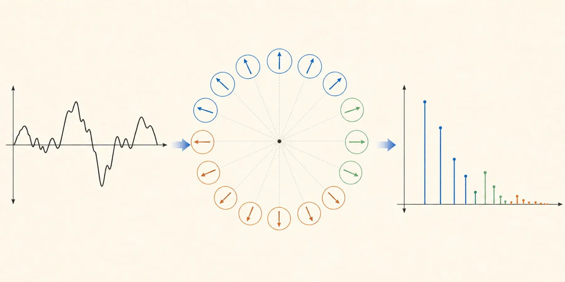
f(x). The equal circles are snapshots of complex test rotations, and the spikes represent frequency contributions in f̂(ξ). This is a conceptual map, not the numerical transform of the particular curve shown. Frequency is a rotation rate across x, not merely one arrow angle.
The Secret of the Dual Worlds
The ultimate magic trick
Most people first meet mathematics in one world: the Shape World, also called the spatial domain. A graph appears, and its bumps, dips, edges, and curves are studied directly.
Fourier analysis opens a second description: the Recipe World, also called the frequency domain. Instead of recording the finished shape point by point, it records which waves make the shape and how strongly each wave contributes.
Here is the secret mathematicians use on problems that seem impossible in the Shape World:
Some problems that are extremely difficult in the Shape World become simple operations in the Recipe World.
The two worlds describe the same mathematical object in different coordinates:
Shape World                         Recipe World

f(x)                               f̂(ξ)
bumps, edges, and locations   ↔     frequencies, strengths, and phases
finished object                    construction recipe
An exact wave recipe needs more than an ingredient list:
frequency     which wave
magnitude     how strongly it appears
phase         where its cycle starts
If phase is discarded, different shapes can share the same frequency magnitudes. The return trip is then not generally exact. The full Fourier transform keeps the complex information needed for reconstruction under the stated inversion assumptions.
The workflow of a genius
- Take the difficult shape.
- Teleport it to the Recipe World with the Fourier transform.
- Perform an easier operation there, such as turning down the high-frequency dial.
- Teleport the result back with the inverse Fourier transform.
- Read the solution in the Shape World.
🌊 difficult shape
        ↓ Fourier transform
🎚️ frequency recipe
        ↓ easy frequency operation
🎵 modified recipe
        ↓ inverse Fourier transform
✨ useful new shape
For example, differentiation is a complicated local operation on a shape, but in the Recipe World it becomes multiplication by iξ:
Exact standard reading:
“The derivative with respect to x of f of x corresponds, under the Fourier transform, to i times xi times f hat of xi.”
The double arrow is read “corresponds to” here. It does not mean that the two expressions are literally equal in the same representation.
Smoothing can become another simple dial:
\[\widehat g(\xi) = m(\xi)\widehat f(\xi),\]Exact standard reading:
“g hat of xi equals m of xi times f hat of xi.”
Here m(ξ) is chosen to weaken high frequencies.
The “teleportation” language is a metaphor. Nothing leaves the mathematical problem. The representation changes. Also, deleting frequencies loses information, so that operation is appropriate for smoothing but not for every theorem. Here “impossible” means difficult in the original representation, not logically impossible.
The helper function: the Magic Color Gate
The teacher rolls a bucket of mixed Lego bricks into the room.
“There are one thousand bricks in here. How many are red?”
Ana reaches into the bucket. “We could inspect them one at a time.”
“Yes,” says Malik, “but we are supposed to be inventors.”
Together they build a conveyor belt with a color scanner and a jar of gold tokens. Every brick passes through the gate exactly once.
Rule card
Rule 1: Inspect one brick at a time.

Rule 2: If the brick is red, drop one token into the jar.

Rule 3: If the brick is not red, drop zero tokens.

Rule 4: After every brick passes, add the tokens.
The first five bricks are:
red   blue   red   yellow   red
 1      0      1      0       1
“Three tokens,” says Ana. “So three of those bricks were red.”
The gate is a helper function. It converts a property into a number. For any property P, define:
The symbol 1_P means “the indicator of P.” It is the mathematical version of the Color Gate:
property true   → 1 → light on
property false  → 0 → light off
Once the detector exists, counting becomes addition:
\[\#\{x:P(x)\} = \sum_x\mathbf{1}_{P}(x).\]Every success contributes 1. Every failure contributes 0.
The story pieces now have exact mathematical jobs:
brick                 input x
red-brick test         property P(x)
token or no token      value 1 or 0
tokens in the jar      sum of indicator values
Prediction round:
If one thousand bricks pass through exactly once and the jar contains 237 tokens, how many bricks passed the red-brick test?
The answer is 237 because every successful test contributes exactly one token.
The Color Gate assumes that the property test is correct and that every object passes exactly once. It packages the bookkeeping, but it does not automatically reduce the amount of computation. It also does not tell us how to construct a difficult test. That is the next problem. A Fourier detector builds such a gate from waves that agree on wanted inputs and cancel algebraically on unwanted inputs.
The exact Fourier parity detector
For every integer n, define:
Exact standard reading:
“E of n equals one plus negative one to the power n, all divided by two. This equals one if n is even and zero if n is odd.”
This is the detector itself. It is an exact finite Fourier function, not merely a game or picture. On the two residue classes modulo 2, its two Fourier notes are the constant character:
and the alternating character:
\[A(n)=(-1)^n.\]The detector is their average:
\[E(n)=\frac{C(n)+A(n)}{2}.\]Why it outputs exactly 1 or 0
If n is even, then n=2k for some integer k. Therefore:
so:
\[E(n)=\frac{1+1}{2}=1.\]If n is odd, then n=2k+1 for some integer k. Therefore:
so:
\[E(n)=\frac{1-1}{2}=0.\]That proves the stated output for every integer. The first few values are:
n:       0   1   2   3   4   5

C(n):    1   1   1   1   1   1

A(n):    1  −1   1  −1   1  −1

E(n):    1   0   1   0   1   0
Agreement becomes a detector
The first Fourier lesson is:
Make waves agree where the helper should be large. Make waves cancel where the helper should vanish.
Here “cancel” means that the represented numbers add to zero. It does not claim that physical energy disappears.
Intuition game: two scorecards
Ana points at the formula. “Can we play the detector before using it in a proof?”
I give the class two scorecards.
Rule 1: The constant card always contributes +1.

Rule 2: The alternating card contributes +1, −1, +1, −1, ...

Rule 3: Add the two contributions and divide by 2.

Rule 4: A final score of 1 opens the gate. A score of 0 closes it.
Prediction round:
What score will the gate produce for
n=12? What aboutn=13?
The rules predict 1 and 0. Substitution into the exact formula verifies both answers.
The scorecards are a way to rehearse the algebra. They do not replace the definition or the proof above.
The detector proves a counting theorem
Claim:
Among the numbers
0, 1, 2, …, 2m−1, exactlymare even.
Use the detector:
\[\sum_{n=0}^{2m-1}E(n) = \sum_{n=0}^{2m-1} \frac{1+(-1)^n}{2}.\]Separate the two parts:
\[\sum_{n=0}^{2m-1}E(n) = \frac{1}{2}\sum_{n=0}^{2m-1}1 + \frac{1}{2}\sum_{n=0}^{2m-1}(-1)^n.\]The first sum contains 2m ones:
The second sum cancels in pairs:
\[1-1+1-1+\cdots+1-1=0.\]Therefore:
\[\sum_{n=0}^{2m-1}E(n)=m.\]The detector did not merely illustrate the answer. It converted the counting problem into a cancellation proof.
The Clock of Cancelling Arrows
The class enters a room with a circular floor and q marked seats:
0 → 1 → 2 → ... → q−1 → 0
At every seat lies a golden arrow of length one. The challenge is:
“Did
nmake a whole number of laps?”
That means:
\[n\equiv0\pmod q.\]Rule card
Rule 1: Every arrow has length 1.

Rule 2: Multiplication by ω rotates an arrow by one q-seat step.

Rule 3: Add arrows head to tail.

Rule 4: A closed polygon has total arrow 0.

Rule 5: Divide the final arrow sum by q.
One arrow-step around the circle is:
\[\omega=e^{2\pi i/q}.\]The powers
\[1,\omega,\omega^2,\ldots,\omega^{q-1}\]are evenly spaced around the unit circle.
Define:
\[\delta_q(n) = \frac{1}{q} \sum_{r=0}^{q-1}\omega^{rn}.\]Exact standard reading:
“Delta sub q of n equals one over q times the sum from r equals zero to q minus one of omega raised to the power r times n.”
Here δ is read “delta,” ω is read “omega,” and the subscript in δq is read “sub q.”
Story reading:
“Spin the
qtest arrows according ton, add them, and divide byq.”
Watch vector addition produce a signal or zero
q=8 example. Alignment finishes far from the start. Eight evenly spaced directions close an octagon and return to zero. The octagon is the coprime case. A nonmatching n that shares a factor with 8 repeats a smaller closed polygon instead, and still sums to zero. With reduced motion enabled, the same conclusion remains visible in the static arrows.
First round: every arrow agrees
Take q=4 and n=0. Every arrow is 1, so every arrow points right:
→ + → + → + → = one arrow of length 4
After division by 4, the score is 1.
Prediction round: can the arrows close?
Keep q=4, but take n=1. The arrows are 1,i,−1,−i. Placed head to tail, they form a square and return to the starting point. The predicted score is 0.
Now try the boundary case n=2. The arrows are 1,−1,1,−1. They trace a two-sided path twice rather than visiting four distinct directions, but they still cancel. This warns us not to assume that every nonmatching input visits every seat exactly once.
Why the clock detector works
Whole laps
If q divides n, then ω^n=1. Every term is 1:
So:
\[\delta_q(n)=1.\]A partial lap
If q does not divide n, set z=ω^n. Then z≠1, but z^q=1. The geometric-sum identity gives:
So:
\[\delta_q(n)=0.\]We have proved:
\[\delta_q(n) = \begin{cases} 1,&q\mid n,\\ 0,&q\nmid n. \end{cases}\]The arrows explain the same result visually:
q divides n       every arrow aligns                 sum q
q does not divide n
                  a nontrivial polygon closes,
                  possibly after repeated smaller loops       sum 0
This is a finite form of character orthogonality: matching rhythms survive a complete average, while nonmatching characters sum to zero.
The story has an exact boundary. The arrows are complex numbers represented as vectors, not physical forces. Cancellation means their vector sum is zero. The geometric-sum identity is the proof, and the picture predicts its two cases.
Count solutions by inserting the detector
Suppose we want to count pairs (x,y) with:
The detector turns the condition into a number:
\[N = \sum_{x=0}^{q-1} \sum_{y=0}^{q-1} \delta_q(x+y).\]Substitute the Fourier detector:
\[N = \frac{1}{q} \sum_{r=0}^{q-1} \sum_x\sum_y \omega^{r(x+y)}.\]The exponent splits:
\[\omega^{r(x+y)} = \omega^{rx}\omega^{ry}.\]So the two sums separate:
\[N = \frac{1}{q} \sum_{r=0}^{q-1} \left(\sum_x\omega^{rx}\right) \left(\sum_y\omega^{ry}\right).\]When r=0, each inner sum equals q.
When r≠0, the arrows complete a nontrivial circle and cancel, so each inner sum is 0.
Only one frequency survives:
\[N = \frac{1}{q}(q)(q) =q.\]There are exactly q solutions.
The teacher circles the proof:
logical condition
      ↓ detector
sum of waves
      ↓ cancellation
exact count
The Spin Lock: extract one hidden frequency
Fourier functions can also act as precise listening devices.
The teacher places a spinning compass on the table. “Every pure note rotates at its own integer speed. The lock opens only when the test wheel removes exactly that rotation.”
Suppose the finite wave mixture is:
\[F(x) = \sum_{k=-N}^{N}c_ke^{ikx}.\]The coefficient c_k records both magnitude and phase. The challenge is to recover one chosen coefficient c_m without disturbing the others.
Rule card
Rule 1: The note eⁱᵏˣ rotates k times during one complete 2π round.

Rule 2: The test wheel e⁻ⁱᵐˣ rotates backward m times.

Rule 3: Multiplying the wheels subtracts their rotation counts.

Rule 4: Average the resulting arrow over exactly one complete round.

Rule 5: A stationary arrow survives; a nonzero integer rotation closes and averages to 0.
First round
Test the note e^{i5x} with the reverse wheel e^{-i5x}:
The arrow stops rotating. Its full-round average is 1.
Prediction round
Test the same note with e^{-i3x}:
The remaining arrow makes two complete rotations. Its path closes, so its full-round average is 0.
The exact rule is:
\[\frac{1}{2\pi} \int_0^{2\pi} e^{ikx}e^{-imx}\,dx = \begin{cases} 1,&k=m,\\ 0,&k\ne m. \end{cases}\]Apply that rule to the whole mixture:
\[c_m = \frac{1}{2\pi} \int_0^{2\pi} F(x)e^{-imx}\,dx.\]Every mismatched integer frequency averages to zero. Only the stationary matching term remains. This is orthogonality in action, and it proves that a finite Fourier description has unique coefficients.
For a real sine-and-cosine description, the same mechanism gives:
\[a_m = \frac{1}{\pi} \int_0^{2\pi}F(x)\cos(mx)\,dx, \qquad b_m = \frac{1}{\pi} \int_0^{2\pi}F(x)\sin(mx)\,dx\]for m≥1, with the constant term handled separately.
The lock has limits. Exact cancellation here uses integer frequencies and a complete 2π interval with the stated averaging measure. A shorter observation window can produce spectral leakage. Also, an opposite-phase copy of the same frequency is not orthogonal: it produces a negative surviving coefficient rather than zero.
The Codebreaker’s Rhythm Test
Malik brings the class a message encrypted by a toy repeating-key cipher.
“The letters look mixed up,” he says. “Can Fourier analysis read the message?”
“Not directly,” I answer. “First it can help us search for a repeating rhythm hidden underneath the letters.”
Imagine that the cipher uses three masks over and over:
position     0 1 2 3 4 5 6 7 8 ...
key mask     A B C A B C A B C ...
The encrypted letters vary, but the schedule of masks repeats every three positions.
Rule card
Rule 1: Give each possible ciphertext symbol its own 0-or-1 indicator strip.

Rule 2: Compare the strips with shifted copies of themselves.

Rule 3: A shift that repeatedly aligns the same key positions may receive a larger coincidence score.

Rule 4: Use a discrete Fourier transform to inspect or compute those periodic correlations.

Rule 5: Treat a peak as a candidate period, not as decoded plaintext.
For ciphertext symbol a, define a length-L indicator strip:
Exact standard reading:
“I sub a of j equals one if ciphertext position j contains a, and equals zero otherwise.”
Assume in this finite game that L is a multiple of the toy key period, so cyclic wraparound preserves the lanes. The total coincidence score at shift s is:
Exact standard reading:
“C of s equals the sum over a of the sum from j equals zero to capital L minus one of I sub a of j times I sub a of the quantity j plus s modulo capital L.”
The words “modulo capital L” mean that the shifted position wraps around the finite strip.
Prediction round
If the toy key repeats every three positions, which shift is more likely to compare positions encrypted by the same key mask: s=1 or s=3?
The rule card predicts s=3. Positions 0,3,6,… form one lane, positions 1,4,7,… form another, and positions 2,5,8,… form the third.
Fourier analysis connects the indicator strips to the coincidence scores. Define:
\[X_a(k) = \sum_{j=0}^{L-1} I_a(j)e^{-2\pi i k j/L}\]Exact standard reading:
“X sub a of k equals the sum from j equals zero to capital L minus one of I sub a of j times e to the power negative two times pi times i times k times j, all divided by capital L.”
and combine their power spectra:
\[P(k)=\sum_a\lvert X_a(k)\rvert^2.\]Exact standard reading:
“P of k equals the sum over a of the absolute value of X sub a of k, squared.”
The bars in |Xa(k)| mean complex absolute value, also called magnitude. The exponent 2 squares that magnitude.
Then the inverse discrete Fourier transform recovers the cyclic coincidence scores:
\[C(s) = \frac{1}{L} \sum_{k=0}^{L-1} P(k)e^{2\pi i k s/L}.\]Exact standard reading:
“C of s equals one over capital L times the sum from k equals zero to capital L minus one of P of k times e to the power two times pi times i times k times s, all divided by capital L.”
A repeating structure can therefore appear as peaks in a correlation plot or as concentrated spectral energy at related frequencies. Once a candidate period p is found, split the ciphertext into p lanes. For a Vigenère-style toy cipher, each lane behaves like a Caesar cipher, so ordinary letter-frequency counts can test candidate shifts inside that lane.
The two kinds of frequency analysis have different jobs:
Fourier or correlation analysis   search for repeating positions
letter-frequency analysis         compare symbol counts inside each lane
The game has strict limits. A peak is statistical evidence, not proof of the key length. Short messages, accidental repetitions, or nearly uniform source text can create weak or misleading results. Encoding letters as arbitrary numbers can also create artificial spectra, which is why the construction used one indicator strip per symbol. Strong modern encryption is designed not to expose useful periodic or frequency structure, and Fourier analysis alone does not recover meaning or plaintext.
The Spotlight Workshop: build a soft detector
A detector is sharp. Sometimes a proof needs a soft spotlight:
bright near the target
dim far away
never negative
total brightness known
Noor dims the room. “Can we make the light gather near one point without allowing negative brightness?”
Rule card
Rule 1: Add N equal wave arrows.

Rule 2: Aim them so they all align at the target x=0.

Rule 3: Square the bundle's size so brightness cannot be negative.

Rule 4: Divide by N so the total normalized brightness remains 1.
Start with a wave bundle:
\[G_N(x) = 1+e^{ix}+e^{2ix}+\cdots+e^{i(N-1)x}.\]At x=0, every wave equals 1, so all arrows align:
Away from 0, the arrows point in different directions and begin to cancel.
Now square the size:
\[K_N(x) = \frac{1}{N}\lvert G_N(x)\rvert^2.\]This is the Fejér kernel.
Because it is a squared magnitude:
\[K_N(x)\ge0.\]The total mass is one. To see why, expand:
\[K_N(x) = \frac{1}{N} \sum_{j=0}^{N-1} \sum_{\ell=0}^{N-1} e^{i(j-\ell)x}.\]Collect terms having the same difference k=j−ℓ. Exactly N−|k| pairs have difference k, so:
This formula exposes the spectral cost of the square. The bundle G_N uses frequencies 0,...,N−1, while |G_N|² uses every difference frequency from −(N−1) through N−1.
Average over one period. Every term with j≠ℓ cancels. The N terms with j=ℓ each contribute 1:
A spotlight made from aligned waves
As N grows, the kernel keeps total mass one but concentrates more of that mass near x=0.
Prediction round:
If the total brightness stays fixed while the beam becomes narrower, what must happen near its center?
The center becomes taller. Indeed, K_N(0)=N. The game predicts the height before the formula confirms it.
That gives us a soft version of a detector:
exact detector     1 here, 0 there
spotlight          mostly here, very little there
The spotlight is not an exact point detector at any finite N. It still has light away from the center. The theorem below needs a limit and continuity assumptions to turn increasing concentration into uniform approximation.
The spotlight proves an approximation theorem
Let f be a continuous 2π-periodic function. Define:
This is a weighted average of nearby values of f.
The Fejér approximation theorem says:
\[\sup_{x\in\mathbb{R}} \lvert \sigma_Nf(x)-f(x)\rvert \longrightarrow0.\]In words:
The finite Fourier averages
σ_N fapproachfuniformly.
The proof has two rooms.
Near the target
If |y|<δ, continuity makes:
small.
Far from the target
If |y|≥δ, the difference may not be small. But the spotlight places less and less total mass there as N grows.
So:
near region   small change × lots of weight = small
far region    possible change × tiny weight = small
The total error is small.
The formal proof begins with:
\[\sigma_Nf(x)-f(x) = \frac{1}{2\pi} \int_{-\pi}^{\pi} \bigl(f(x-y)-f(x)\bigr)K_N(y)\,dy.\]Then split the integral into |y|<δ and |y|≥δ, and use continuity plus concentration.
This is a powerful proof-engineering lesson:
If the theorem needs a local average, construct a nonnegative, normalized, increasingly concentrated kernel.
When is the square trick complete?
For one-variable trigonometric polynomials, the square construction is more than a convenient sufficient condition. The Fejér–Riesz factorization theorem says that if:
\[T(x)=\sum_{k=-N}^{N}c_ke^{ikx}\]is real-valued and nonnegative for every real x, then there is an ordinary polynomial:
such that:
\[T(x)=\left|P(e^{ix})\right|^2.\]So, in this one-dimensional finite-band setting, searching over squared magnitudes can represent every nonnegative trigonometric polynomial. This statement does not automatically extend to several variables as one squared magnitude. The domain is part of the theorem.
The heat room: filtering frequencies
The class now brings in a rough temperature profile:
🔥░🔥░░🔥░🔥░░░🔥
“Heat should smooth this,” says Noor.
The heat equation is:
\[\frac{\partial u}{\partial t} = \frac{\partial^2u}{\partial x^2}.\]Exact standard reading:
“Partial u over partial t equals partial squared u over partial x squared.”
In meaning, the left side is the partial derivative of u with respect to t, and the right side is the second partial derivative of u with respect to x.
Here u(x,t) is temperature, x is position, and t is time.
For this example, assume x∈ℝ, t>0, and the initial temperature decays enough at infinity for the integrations by parts below to have no boundary terms.
Use the Fourier transform:
\[\widehat u(\xi,t) = \int_{-\infty}^{\infty} u(x,t)e^{-i\xi x}\,dx.\]Exact standard reading:
“u hat of xi comma t equals the integral from minus infinity to infinity of u of x comma t times e to the power negative i times xi times x, d x.”
Fourier analysis turns a second derivative into multiplication:
\[\widehat{\frac{\partial^2u}{\partial x^2}} = -\xi^2\widehat u.\]Exact standard reading:
“The Fourier transform of partial squared u over partial x squared equals negative xi squared times u hat.”
So the heat equation becomes:
\[\frac{\partial\widehat u}{\partial t} = -\xi^2\widehat u.\]Exact standard reading:
“Partial u hat over partial t equals negative xi squared times u hat.”
For each frequency ξ, this is a simple decay equation:
Exact standard reading:
“u hat of xi comma t equals e to the power negative t times xi squared, times u sub zero hat of xi.”
The multiplier is a frequency volume knob:
slow frequency   ξ small   → mostly kept
fast frequency   ξ large   → strongly weakened
Heat mostly keeps slow notes and strongly weakens fast wiggles
The inverse transform gives the Gaussian heat kernel:
\[G_t(x) = \frac{1}{\sqrt{4\pi t}} e^{-x^2/(4t)}.\]Exact standard reading:
“G sub t of x equals one over the square root of the quantity four times pi times t, times e to the power negative x squared divided by the quantity four times t.”
The temperature is:
\[u(x,t) = \int_{-\infty}^{\infty} G_t(y)u_0(x-y)\,dy.\]Exact standard reading:
“u of x comma t equals the integral from minus infinity to infinity of G sub t of y times u sub zero of x minus y, d y.”
This integral is called convolution.
Each source places a shifted Gaussian, then the copies add
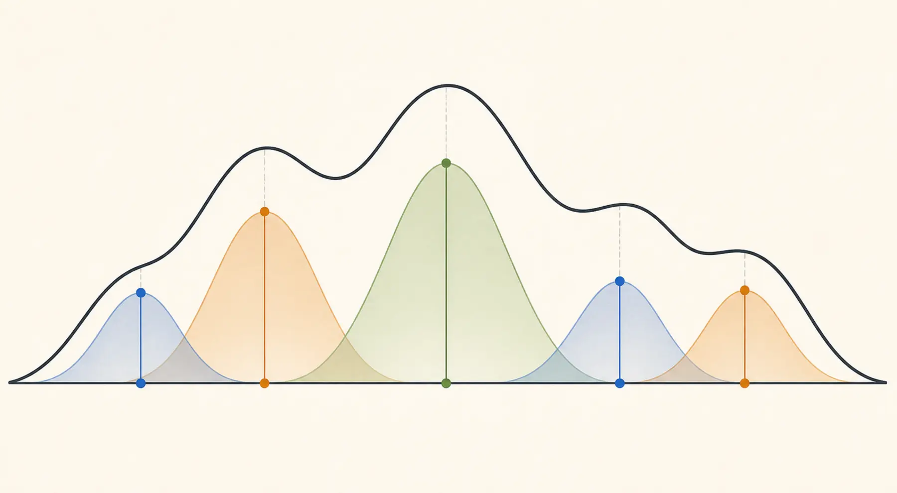
u₀ is five nonnegative weighted point sources. Each colored bell is a translated copy of the same Gaussian, scaled by its source height. The dark curve is their sum. A general u₀ may be continuous or signed, so the integral replaces this finite positive sum.
The Glow Stamp game
Noor replaces a nonnegative temperature line with a dark sheet covered in tiny source points. Beside it sits a translucent stamp shaped like the Gaussian. For signed mathematical data, red and blue ink can represent positive and negative contributions.
Rule card
Rule 1: Every source point places one shifted copy of the same glow stamp.

Rule 2: The source value scales that copy's signed intensity.

Rule 3: Add the contributions from every source point.

Rule 4: Use the same stamp rule at every location.
At output position x, the source at x−y contributes:
Adding continuously over every shift y gives the convolution formula above.
First round:
One idealized point source produces one shifted copy of the Gaussian stamp.
Prediction round:
What do two equal point sources produce?
The rules predict two shifted Gaussian copies added together. Doubling a source doubles its contribution, and shifting every source shifts the final glow by the same amount. These are the linearity and translation rules encoded by convolution.
An asymmetric kernel would create a directional glow. The Gaussian used here is symmetric, so this heat model spreads influence equally left and right.
The picture has a boundary. Literal brightness cannot be negative, so signed functions require the two-color convention. Real ink and thumb smears may also be nonlinear, position-dependent, or irreversible in ways this equation does not model. The Glow Stamp is exact only when shifted, scaled contributions combine linearly according to the declared kernel.
The Gaussian has three proof-friendly properties:
\[G_t(x)\ge0,\] \[\int_{-\infty}^{\infty}G_t(x)\,dx=1,\]and:
\[G_t\text{ is smooth for }t>0.\]Therefore the later temperature is an average of nearby starting temperatures. It does not create a new value larger than the largest starting value:
\[\lvert u(x,t)\rvert \le \sup_y\lvert u_0(y)\rvert.\]The frequency design explains the smoothing. The kernel shape makes the averaging properties visible.
There is also a time-composition law:
\[G_t\text{ followed by }G_s = G_{t+s}.\]In frequency space the proof is one line:
\[e^{-t\xi^2}e^{-s\xi^2} = e^{-(t+s)\xi^2}.\]The teacher underlines the pattern:
hard spatial equation
      ↓ Fourier transform
one small equation per frequency
      ↓ solve
frequency multiplier
      ↓ inverse transform
proof-friendly spatial kernel
Can a program automate this?
The class writes a program card:
🧠 human states the proof goal
🧮 program chooses a search space
🎚️ program searches for coefficients
🔄 program reconstructs a candidate function
🔍 checker verifies the certificate
📜 human connects the properties to the theorem
The honest answer is:
Yes, function engineering can be automated inside a declared family. The program can search for a candidate. A separate checker must still verify the mathematical obligations.
The bounded synthesis version
Suppose the program is allowed to use only these waves:
\[1,\cos(x),\sin(x),\ldots,\cos(Nx),\sin(Nx).\]The unknowns are the coefficients:
\[a_0,a_1,b_1,\ldots,a_N,b_N.\]The proof goal becomes constraints on those numbers:
detector:
  value = 1 at the target
  value = 0 at the forbidden inputs

spotlight:
  value ≥ 0
  total mass = 1
  mass outside the target region is small

filter:
  low frequencies survive
  high frequencies shrink
The program can then use:
linear algebra          exact linear constraints
linear programming      inequalities on coefficients
symbolic algebra        identities and simplification
sum-of-squares methods  some positivity searches
interval arithmetic     certified numerical bounds
The solver proposes coefficients. The checker expands the resulting function and verifies each promised property.
If positivity is encoded by writing K=|G|², the search must also account for the enlarged difference-frequency support of K. Positivity is gained, but bandwidth is spent.
A bounded Fourier synthesis loop
A small numerical experiment
This program evaluates the modular detector with floating-point complex numbers:
from cmath import exp, pi


def fourier_detector(n, q):
    omega = exp(2j * pi / q)
    return sum(omega ** (r * n) for r in range(q)) / q


for q in range(2, 9):
    for n in range(2 * q):
        expected = 1 if n % q == 0 else 0
        value = fourier_detector(n, q)
        assert abs(value - expected) < 1e-10
This is useful evidence. It checks a finite collection of examples.
It is not, by itself, a proof for every integer n and every q. The proof is the geometric-sum identity, which handles the unbounded claim symbolically.
A proof-carrying automation loop
A safer program returns more than a picture:
candidate coefficients
      +
domain and assumptions
      +
exact identities
      +
error or positivity bounds
      ↓
finite proof certificate
      ↓
independent checker
The checker should be able to reject:
wrong domain
missing normalization
unverified continuous claim
floating-point error mistaken for zero
frequency family too small for the requested shape
This separates four jobs:
finding a candidate  = search
showing a picture    = explanation
deriving properties  = proof
replaying the steps   = checking
What automation cannot promise automatically
A solver does not become an oracle merely because it uses Fourier coefficients.
It may find a function that works on sampled points but fails between them.
It may find a positive value at many points without proving positivity on the whole interval.
It may solve a finite optimization problem while the theorem asks about an infinite family.
It may return a floating-point number that is close to zero but not exactly zero.
The safe claim is conditional:
If the search space is specified and the checker verifies the required analytic properties, automation can produce a proof-carrying helper function for that problem.
The backward-design worksheet
The teacher gives each child a card.
The proof goal
What must the helper function do?
detect
count
cancel
concentrate
smooth
bound
solve a differential equation
The spatial promises
nonnegative?
localized?
integral one?
specific zeros?
bounded?
symmetric?
smooth?
The frequency promises
which frequencies exist?
how loud is each one?
which phases make them align?
which frequencies must disappear?
how quickly should high frequencies decay?
The construction move
positivity        → square the magnitude, then count the new frequencies
mass one          → normalize
concentration     → align many frequencies
exact cancellation → use a complete cycle
smoothing         → suppress high frequencies
extract one note  → multiply by its reverse wave and average a complete period
convolution       → shift, scale, and add copies of one declared kernel
The verification move
check the formula
check the domain
check normalization
check convergence or error
check the final theorem bridge
The helper function is not complete until every promise has a proof.
Three common traps
A positive spectrum is not automatically a positive shape
The fact that f̂(ξ)≥0 does not, by itself, guarantee f(x)≥0.
If spatial positivity is needed, a safer design is often:
\[K(x)=\lvert G(x)\rvert^2.\]Squaring the magnitude gives a direct reason for K(x)≥0.
In one variable and with finite frequency support, Fejér–Riesz factorization explains why this search form is complete for nonnegative trigonometric polynomials. Outside that setting, it is only a justified construction family, not a universal promise.
Finite tests are not continuous proofs
Checking a function at one thousand points does not prove a statement about every real input. A continuous proof needs a bound between sample points, a symbolic identity, or another certificate that covers the entire domain.
The domain changes the Fourier tool
finite clock      finite Fourier sums
periodic circle   Fourier series
real line         Fourier transform
heat flow         frequency multiplier plus inverse transform
The notation may look similar while the theorem changes. Always name the world before using the formula.
The pocket map
The class compresses the lesson:
📖 story
      ↓
🎮 exact rules
      ↓
🧩 worked round
      ↓
💡 prediction
      ↓
📐 formula
      ↓
✅ proof and boundary
The story helps generate a prediction. The formula and proof decide whether that prediction is true.
The proof-engineering pipeline is:
🎯 proof job
      ↓
🎵 frequency design
      ↓
🔄 Fourier synthesis
      ↓
🌊 helper function
      ↓
🔍 verified properties
      ↓
📜 theorem
The three central constructions are:
exact detector
  waves align on the target
  waves cancel away from it

soft spotlight
  square a wave bundle
  normalize its total mass
  add frequencies to concentrate it

heat filter
  keep slow frequencies
  suppress fast frequencies
  transform back into a smoothing kernel

spin lock
  multiply by a reverse test frequency
  average over the declared complete period
  keep only the stationary match

codebreaker rhythm test
  build one indicator strip per symbol
  use correlation or Fourier peaks to propose a period
  split into lanes before ordinary symbol counting

glow stamp
  shift one kernel to every source location
  scale each copy by the source value
  add all contributions
The deepest sentence is:
Fourier proof design means building a mathematical tool from waves: make the waves agree where strength is wanted, cancel where zero is wanted, weaken the frequencies that must disappear, and verify the resulting function before using it.
The program can help search.
The picture can help explain.
The certificate can help check.
The theorem still depends on the verified bridge between the helper function and the claim.
Part II: fewer knobs, smaller search
The next afternoon, the teacher brings a machine with many knobs.
“A Fourier function may have many adjustable coefficients,” I say. “A computer can search them, but it helps to remove choices that the proof does not need.”
Malik asks, “Is removing choices the same as proving?”
“No. Removing choices can make a search smaller. It is safe only when we know that a solution has not been removed.”
That is the second lesson:
Reduce the search space, but prove that the reduction is allowed.
Fewer knobs, smaller search
A degree of freedom is a choice
A degree of freedom is one independent choice.
Think of a machine with three knobs:
🎛️ knob a
🎛️ knob b
🎛️ knob c
Start with:
\[f(x)=a+bx+cx^2.\]The knobs control:
a   height
b   tilt
c   curve
Before adding any rules, a, b, and c can be chosen independently. There are three degrees of freedom.
Now require:
\[f(0)=0.\]Since f(0)=a, the rule forces:
One knob is locked:
before:   🎛️a   🎛️b   🎛️c

after:    🔒a=0  🎛️b   🎛️c
Add a second rule:
\[f(1)=1.\]Then:
\[b+c=1.\]The two knobs b and c are no longer independent. Choose b, and c=1-b is forced.
The search has changed:
3 free choices
      ↓ f(0)=0
2 free choices
      ↓ f(1)=1
1 free choice
The equations have not yet selected one function. They have made the remaining search smaller.
Fourier coefficients are knobs
A periodic function may be written formally as:
\[f(x)=\sum_{k=-\infty}^{\infty}a_ke^{ikx}.\]Each a_k controls one frequency.
a₋₂   frequency −2
a₋₁   frequency −1
a₀    constant note
a₁    frequency 1
a₂    frequency 2
An unrestricted Fourier description has infinitely many knobs. A program cannot simply try every real sequence of coefficients.
So begin with a declared finite family:
\[f_N(x) = \sum_{k=-N}^{N}a_ke^{ikx}.\]For N=2, this is a five-coefficient search:
This is called band-limited in this finite sense. The family uses only a limited band of notes.
The reduction is useful, but it has a boundary:
If the real helper needs frequency
7, a search restricted to frequencies0,1,2will not find it.
Failure inside a small family proves only:
no candidate was found in this box
It does not prove:
no candidate exists anywhere
Real-valued functions pair their notes
The complex Fourier coefficients of a real-valued function obey:
\[a_{-k}=\overline{a_k}.\]The bar means complex conjugation, which reflects a rotating arrow across the real axis.
This pairing removes duplicate choices. The same real function can be written using cosines and sines:
\[f(x) = a_0+ \sum_{k=1}^{N} \bigl(b_k\cos(kx)+c_k\sin(kx)\bigr).\]Now the knobs are real coefficients a_0,b_k,c_k.
Symmetry removes more knobs
Suppose the desired helper is even:
\[f(-x)=f(x).\]It has mirror symmetry around zero:
             /\
          __/  \__
_________/        \_________
       −x          x
Sine is odd:
\[\sin(-x)=-\sin(x).\]Therefore an even Fourier sum has no sine terms:
\[f(x) = a_0+\sum_{k=1}^{N}b_k\cos(kx).\]The reduction ladder is:
all functions
      ↓ choose a finite band
finite Fourier sums
      ↓ require real values
sine and cosine sums
      ↓ require even symmetry
cosine sums only
Fewer knobs mean a smaller search. The reduction is safe only if the theorem’s helper can be replaced by an even helper without losing the required properties.
Averaging can make symmetry safely
Suppose f is a candidate. Build its mirror-average:
Then:
\[f_{\mathrm{even}}(-x)=f_{\mathrm{even}}(x).\]The averaging operation has forced even symmetry.
But a proof obligation remains:
Do the properties needed by the theorem survive this averaging?
For example, linear equalities often survive averaging. A nonlinear condition may not. A positivity condition does survive if both f(x) and f(-x) are nonnegative, because an average of nonnegative numbers is nonnegative.
This is the difference between:
safe reduction:
  prove a solution can be symmetrized

unsafe reduction:
  search symmetric functions because they look convenient
A tiny three-knob spotlight
The teacher asks for a function with:
✅ height 1 at x = 0
✅ height 0 at x = π
✅ no negative values
✅ only a few frequencies
Start with:
\[K(x)=a+b\cos(x)+c\cos(2x).\]There are three knobs:
🎛️ a
🎛️ b
🎛️ c
The first condition gives:
\[K(0)=a+b+c=1.\]The second gives:
\[K(\pi)=a-b+c=0.\]Subtract the second equation from the first:
\[2b=1, \qquad b=\frac12.\]Then:
\[a+c=\frac12.\]Two equations have reduced three knobs to one free choice. They have not yet proved positivity.
To see the entire remaining family, write:
\[y=\cos(x), \qquad -1\le y\le1,\]and use cos(2x)=2y²−1. Since b=1/2 and a=1/2−c:
The first factor is nonnegative on [-1,1]. The second factor is affine, so its minimum occurs at an endpoint. Exact endpoint checking gives:
This exposes an important point: the original conditions do not select a unique spotlight. They select a whole half-line of valid coefficients.
For a falsifier, choose c=1/7 and y=−7/8. Then:
So a candidate just beyond the boundary really does fail between the two required endpoints.
The boundary choice c=1/8 has an extra property. It makes K''(π)=0, producing the flattest zero at π within this family. Equivalently, it maximizes c subject to nonnegativity. That additional design rule selects the square:
This immediately gives:
\[K(x)\ge0.\]It also gives:
\[K(0)=1, \qquad K(\pi)=0.\]Expand the square:
\[K(x) = \frac{(1+\cos(x))^2}{4}.\]Using:
\[\cos^2(x)=\frac{1+\cos(2x)}{2},\]we obtain:
\[K(x) = \frac38+\frac12\cos(x)+\frac18\cos(2x).\]So the exact coefficients are:
\[a=\frac38, \qquad b=\frac12, \qquad c=\frac18.\]The square was more than a pretty formula. It carried positivity inside the construction. The new extremal condition explains why this square was selected from the other valid choices.
How much did the search shrink?
Imagine each coefficient can take ten trial values.
With six independent coefficients:
\[10^6=1,000,000\]candidates exist.
If symmetry removes three degrees of freedom, only three remain:
\[10^3=1,000\]candidates remain.
6 knobs   → 1,000,000 trial combinations
3 knobs   →       1,000 trial combinations
The search is one thousand times smaller.
This is not a proof that the reduced family contains the answer. It is a proof-engineering benefit conditional on the reduction being sound.
What programs do
Fourier proof work uses programs at several levels:
human:
  chooses the theorem and the meaning

program:
  computes transforms
  searches coefficients
  solves equations
  plots candidates
  estimates or certifies bounds

checker:
  replays exact identities
  accepts or rejects the certificate
The Fast Fourier Transform
Suppose a program receives sampled values:
[3, 4, 6, 4, 3, 1, 0, 1]
The Fast Fourier Transform, or FFT, quickly converts those samples into frequency data:
sampled shape
      ↓ FFT
frequency strengths
The FFT is an efficient calculation. It does not by itself prove a theorem about every real input.
Coefficient search
For a family such as:
\[K(x)=a_0+a_1\cos(x)+\cdots+a_N\cos(Nx),\]a program can search for coefficients satisfying:
K(0)=1
K(π)=0
K(x) ≥ 0
small mass away from zero
Different constraints suggest different tools:
linear equations        exact linear algebra
linear inequalities     linear programming
polynomial positivity   symbolic or sum-of-squares methods
continuous bounds       interval arithmetic
large numerical search  optimization
The solver proposes a candidate. The checker must then verify every property used by the theorem.
Numerical search is discovery, not automatic proof
A program may report:
minimum value ≈ 0.0000003
That does not automatically prove:
\[K(x)\ge0 \qquad\text{for every real }x.\]The graph may have missed a dip between sample points. Floating-point rounding may have hidden a small negative value. The optimizer may have stopped at a local solution.
The four levels of computer help are:
1. exploration
   plots and examples

2. numerical search
   candidate coefficients

3. rigorous numerical certification
   intervals and error bounds

4. formal proof checking
   exact replay of a certificate
The level must be named. “The computer found it” is not a proof category.
Interval arithmetic
Ordinary arithmetic may say:
the answer is approximately 0.37
Interval arithmetic says:
\[x\in[0.369,0.371].\]The interval is guaranteed to contain the true value.
To certify K(x)≥0 on a whole interval:
split the domain
      ↓
bound K on every small piece
      ↓
every lower bound is ≥ 0
      ↓
K is ≥ 0 everywhere
The certificate is a collection of boxes and verified bounds.
Exact algebra after numerical discovery
A numerical search may return:
a ≈ 0.3750000001
b ≈ 0.4999999998
c ≈ 0.1250000000
A person may recognize:
\[a=\frac38, \qquad b=\frac12, \qquad c=\frac18.\]The final proof should use the exact fractions and prove the identity. A decimal guess is a clue, not the certificate.
The three-seat detector, redesigned by a program
Suppose the program must detect multiples of 3. The three residues are:
0 → 1
1 → 0
2 → 0
Let:
\[\omega=e^{2\pi i/3}.\]Search for:
\[D(n)=a+b\omega^n+c\omega^{2n}.\]The desired outputs create the equations:
\[a+b+c=1,\] \[a+b\omega+c\omega^2=0,\] \[a+b\omega^2+c\omega=0.\]The exact solution is:
\[a=b=c=\frac13.\]Therefore:
\[D(n) = \frac13\bigl(1+\omega^n+\omega^{2n}\bigr).\]The program solved the coefficient system. Fourier cancellation explains why the solution works for every integer n.
The degree count is:
3 coefficient knobs
− 3 independent output conditions
= 0 free knobs
Enough correct conditions can force a unique helper.
A program-assisted proof pipeline
The class draws the complete machine:
🎯 theorem
      ↓
🧠 semantic design
What kind of helper would force it?
      ↓
✂️ justified reduction
symmetry, finite band, normalization
      ↓
💻 computer search
find promising coefficients
      ↓
🔢 exact recovery
turn decimal patterns into exact values
      ↓
📜 proof
show the helper has the required properties
      ↓
🤖 certification
replay the finite certificate
      ↓
✅ theorem
The boundary of automation
A program can search a declared family and certify declared obligations. It does not automatically choose the right theorem, justify an unsafe reduction, or turn finite samples into a statement about every real input.
This is the same separation used in formal methods:
search        proposes a candidate
explanation   shows the picture
proof         derives the required facts
checker       replays the public steps
A majorant can build an inequality proof
Sometimes the helper should sit above a difficult function.
If:
\[F(x)\le K(x)\]and:
\[K(x)\le B,\]then:
\[F(x)\le K(x)\le B.\]The function K is a majorant, an easy roof over F. A function below F is a minorant.
The computer can search for a Fourier-built roof:
hard function F
       ↓ below
easy Fourier roof K
       ↓ below
constant ceiling B
If the goal asks for the best possible ceiling, the search becomes an extremal problem:
valid helper functions
      ↓ optimize
best helper
      ↓
sharp bound
Finding a good helper is only half of an optimality proof. The proof must also show that no valid helper can do better.
Convex and nonconvex searches
Some coefficient searches form a convex problem. Child picture:
convex bowl:

        \        /
         \      /
          \____/
In a convex problem, a locally optimal point is globally optimal under the stated assumptions. This can make certification easier.
Other searches have many valleys:
\__/\/\____/\__/
A numerical optimizer may stop in one valley without finding the best one.
So a rigorous report should say:
what family was searched
what constraints were enforced
what objective was optimized
whether the solver found a global or local result
how the final candidate was certified
Four small exercises
Build the odd-number lamp
Construct a function that returns 1 for odd n and 0 for even n.
Hint:
\[O(n)=1-E(n) = \frac{1-(-1)^n}{2}.\]Ask:
Why do the waves agree on odd numbers?
Why do they cancel on even numbers?
Remove a sine family
Start with a candidate f. Build:
Prove that f_even is even. Then list one theorem property that survives averaging and one nonlinear property that might not.
Classify the three-note spotlights
Start with:
\[K(x)=a+b\cos(x)+c\cos(2x).\]Require:
\[K(0)=1, \qquad K(\pi)=0.\]Find the remaining one-parameter family. Prove that it is nonnegative exactly when c≤1/8. Then show that requiring K''(π)=0 selects:
Expand it and verify nonnegativity.
Separate search from proof
Write one sentence for each:
What did the program search?
What exact statement did the checker verify?
What theorem bridge still needed a human proof?
Part II in one picture
huge function space
          ↓ justified constraints
small Fourier family
          ↓ computer search
promising coefficients
          ↓ exact pattern recovery
mathematical candidate
          ↓ independent checker
proof certificate
          ↓ theorem bridge
proved conclusion
The teacher closes the knob machine.
“Reducing degrees of freedom makes a search smaller,” I say. “It does not make an unjustified assumption true.”
Ana points to the Fourier detector.
“So the safest order is?”
The class answers:
name the theorem
choose what the helper must do
reduce only with a reason
search the remaining knobs
recover exact mathematics
check every promise
connect the helper to the theorem
The final sentence is:
A small search can discover a proof function, but only a justified reduction and an independent certificate can turn the discovery into a theorem.
Part III: a tiny proof-carrying lab
The class now gives the three-note problem to a small deterministic checker.
The checker does not sample a graph. It receives a rational value of c and verifies four finite obligations:
1. substitute b = 1/2 and a = 1/2 − c
2. expand the claimed factorization exactly
3. check K(1) = 1 and K(−1) = 0 in the y-coordinate
4. minimize the remaining affine factor by checking the correct endpoint
The source is:
examples/fourier_function_engineering/verify_three_note_spotlight.py
Run:
python3 examples/fourier_function_engineering/verify_three_note_spotlight.py
The self-test includes:
c = 1/8    accepted, extremal square
c = 0      accepted, proving nonuniqueness
c = −2     accepted, another valid member
c = 1/7    rejected with the exact witness y = −7/8
This is a narrow checker, not a general theorem prover. Its authority is deliberately small:
search or human proposes c
          ↓
exact checker verifies this declared family
          ↓
the tutorial proves why the finite checks cover every x
The key bridge is the substitution y=cos(x). It turns an infinite trigonometric claim into a polynomial claim on the compact interval [-1,1]. The factorization then reduces positivity to one affine endpoint check.
That is Fourier function engineering in miniature:
shape requirement
      ↓
frequency family
      ↓
algebraic reparameterization
      ↓
small exact certificate
      ↓
independently checked claim
The lab does not prove that this spotlight is best for every theorem. It proves exactly which members of this declared three-note family satisfy the stated constraints, and why.
Further reading
- On a Fejér–Riesz factorization of generalized trigonometric polynomials states the classical one-variable factorization and develops a generalized version.
- Factorization of multivariate positive Laurent polynomials explains why several variables require a more careful sum-of-squared-magnitudes theory.